
Simulation modeling plays a crucial role in comprehending and analyzing intricate systems, as it enables engineers, scientists, and researchers to simulate and predict their behavior. Discrete event simulation is a popular technique in simulation modeling, where the simulation model progresses by a sequence of events that happen at distinct points in time. However, when the system dynamics are dictated by continuous processes instead of discrete events, discrete event simulation may not be the most appropriate approach. In such cases, time-driven simulation can be a valuable alternative that provides a more accurate model of the system’s behavior.
What is Time Driven Simulation?
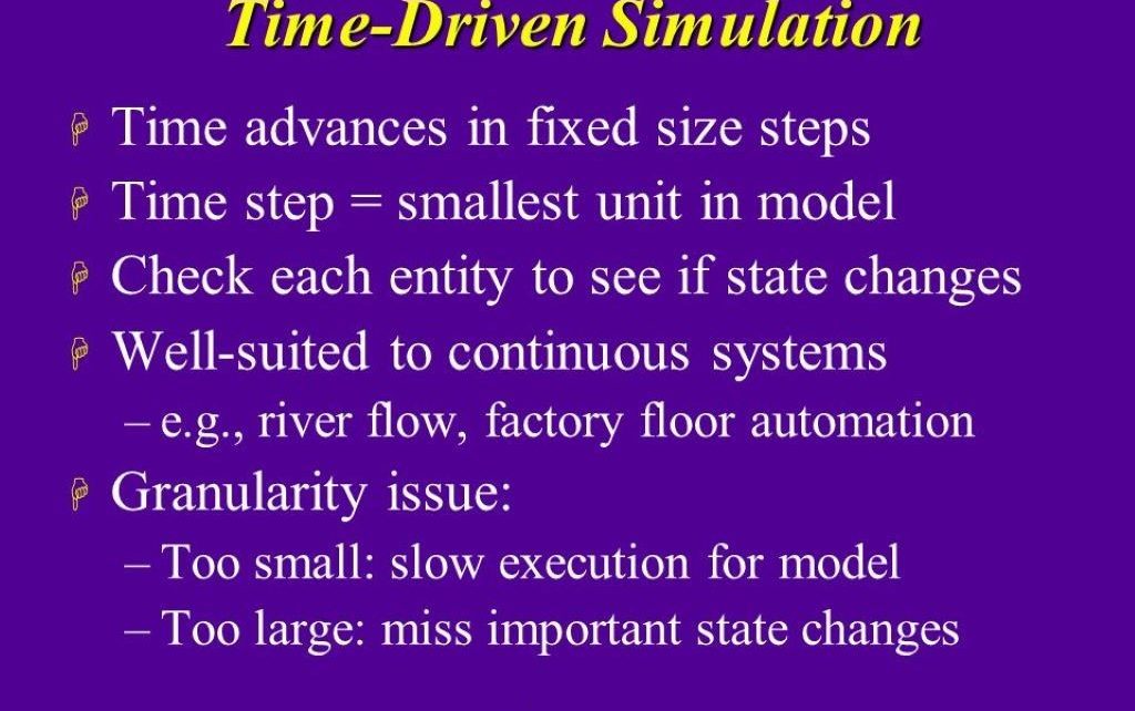
Time driven simulation is a simulation modeling technique where the state of the system is updated at regular discrete time intervals, rather than being triggered by events. In this approach, time progresses in fixed incremented steps, and the system equations are solved at each time step to compute the new state of the system.
The key characteristics of time driven simulation are:
- Time progresses in fixed discrete steps
- System equations are solved at each time step
- System state is updated every time step
This is in contrast to discrete event simulation, where time jumps to the next event occurrence and system state changes only at event times.
Some key advantages of time driven simulation are:
- Handles continuous system dynamics well
- Easier to model complex interdependent processes
- Suitable for modeling high frequency dynamics
Time driven simulation is commonly used for modeling engineering systems that have frequent or continuous dynamics, such as control systems, communication networks, analog circuits, and mechanical systems with rigid body dynamics.
Time Driven vs Discrete Event Simulation
The main differences between time driven and discrete event simulation are summarized below:
- Progression of time:
- Discrete event: Time jumps to next event
- Time driven: Time progresses in fixed steps
- System state updates:
- Discrete event: Only at event times
- Time driven: Every time step
- System dynamics:
- Discrete event: Governed by discrete sequence of events
- Time driven: Can handle continuous dynamics
- Suitable applications:
- Discrete event: Queueing systems, manufacturing, logistics
- Time driven: Control systems, electrical networks, rigid body mechanics
So in summary, discrete event simulation is best for modeling systems where state changes occur at separate events with significant time gaps in between. Time driven simulation works better for high frequency dynamics and continuous processes.

Time Driven Simulation Methodology
The general procedure for carrying out a time driven simulation study is as follows:
- Develop mathematical model – Develop differential/difference equations describing the system dynamics
- Discretize model equations – Discretize the equations to convert into form suitable for time step-by-step numerical simulation
- Define simulation parameters – Define time step, total time, model inputs, initial conditions, etc.
- Implement simulation – Program the discretized equations in software to iterate the model over time
- Initialize system state – Set the initial conditions
- Advance time – Increment simulation clock by one time step
- Update system state – Use discretized equations to calculate new state variables
- Check end condition – Check if simulation end time reached
- Output results – Record/visualize results for analysis
- Iterate – Go back to Step 6 and repeat until end
The model is initialized, and then the simulation loop runs over and over to march the time forward and update the system state at each time step. The size of the time step determines the accuracy and computational load of the simulation. Smaller time steps yield more accurate results but require more computation time.
Time Step Considerations
Choosing an appropriate time step is an important modeling decision in time driven simulation. The time step affects accuracy, stability, and computational efficiency of the simulation. Some guidelines for selecting time step:
- Should be small enough to capture the system dynamics
- Much smaller than the smallest time constant in the system
- Small enough to maintain numerical stability
- Larger time steps yield lower accuracy but faster runs
- Typical range is 10^-6 to 10^-3 seconds, problem dependent
In some cases, analysts can determine the required time step analytically based on the system mathematics, or they can determine it empirically by running tests to check solution convergence. Alternatively, the simulation can adjust the time step on-the-fly for better accuracy and performance using adaptive time stepping.
Software for Time Driven Simulation
Robust numerical solvers are necessary for time-driven simulation, and developers generally implement it using programming languages like C/C++, Java, Python, etc., instead of relying on simulators designed solely for discrete events. Some commonly used software platforms and tools include:
- MATLAB/Simulink – Widely used platform for modeling and simulating dynamic systems using block diagram models
- Modelica – Object oriented language for modeling physical systems, with open source (OpenModelica) and commercial tools
- Wolfram SystemModeler – Modeling and simulation environment based on Mathematica
- Python – General purpose programming language, with scientific libraries like NumPy, SciPy, matplotlib
- VHDL-AMS – Hardware description language with analog and mixed-signal extensions
- LabVIEW – Graphical programming platform by National Instruments
- 20-sim – Tool specialized for modeling engineering systems based on bond graphs
- AMESim – 1D simulation software tailored for multi-domain mechatronic systems
The choice depends on factors like modeling paradigm, availability, cost, performance, and interoperability with other tools.
Application Areas
Some of the main application areas where time driven simulation is widely used include:
Control Systems
- Modeling closed loop control systems
- Analyzing control loop stability
- Designing and testing controllers before hardware implementation
- Testing control performance for nonlinear systems
Electrical Circuits
- AC and transient circuit analysis
- Modeling analog and mixed signal circuits
- IC and PCB design verification
- Power electronics and motor drives
Multibody Mechanics
- Modeling mechanical systems like vehicles, robots, machinery
- Analyzing rigid body kinematics and dynamics
- Synthesizing and testing mechanical control systems
Hydraulic/Pneumatic Systems
- Modeling fluid power systems in aerospace, automotive, construction equipment
- Analyzing compressibility effects
- Sizing components like cylinders, accumulators
Power Systems
- Modeling generation, transmission and distribution of electric power
- Load flow analysis and transient stability studies
- Design and testing of grid control systems
Communications Networks
- Modeling data traffic and congestion in networks
- Analyzing quality of service and packet transfers
- Testing network control protocols
Chemical Processes
- Modeling reactors, separators, heat exchangers
- Testing control schemes for process variables like pressure, flow rate, temperature
So in summary, time driven simulation is applicable to a wide range of engineering domains involving dynamic systems and physical processes that are continuous or high frequency in nature. It allows modeling complex interdependencies between components and analyzing transient performance.
Hybrid Simulation
In some cases, a system may involve both time-driven and discrete event dynamics. For example, a manufacturing production line with continuous material flow as well as discrete control logic and events. Such systems can be modeled using hybrid simulation techniques:
- Parallel DE and TD: Discrete event and time driven simulators run in parallel with data exchange at synchronization points
- TD simulation with DE events: Time driven simulator able to handle both continuous states and discrete events
- Quantized TD: Time driven model that approximates events by quantizing states into discrete values
Hybrid simulation provides flexibility to model complex systems using suitable techniques for each subsystem while enabling interaction between the different parts.
Advantages of Time Driven Simulation
Some of the main advantages of time driven simulation are:
- Handles continuous system dynamics accurately
- Can model very high frequency systems
- Better for complex interdependent processes
- Easier to incorporate complex mathematical models
- Facilitates modeling across different engineering domains
- Interfaces well with physical system testing using hardware-in-the-loop
- Supports nonlinearities, higher order systems, and stiff systems
- Time step provides a control for tradeoffs between accuracy and speed
Challenges with Time Driven Simulation
Some of the main challenges associated with time driven simulation include:
- Requires robust numerical integration solvers
- Can have stability issues for stiff systems
- Generally more computationally intensive than discrete event
- Time step needs to be properly selected for accuracy and performance
- Algebraic loops require special handling
- Difficult to model discontinuous or non-differentiable dynamics
- Requires greater programming expertise compared to simulators
- Debugging complex models can be difficult
So in summary, while time driven simulation provides significant modeling flexibility and accuracy, it also entails greater complexity in implementation compared to less computationally intensive approaches like discrete event.
Trends and New Developments
Some of the trends and recent developments related to time driven simulation include:
- Growing use of time driven simulation in cyber-physical systems design
- Increasing adoption in autonomous systems like robots, self-driving cars
- Integration with artificial intelligence for neural network modeling
- Hybrid simulation combining time driven and discrete event models
- Use of parallel and cloud computing to speed up simulations
- Better numerical algorithms for stiff systems and algebraic loops
- Tighter integration with hardware-in-the-loop testing
- Standardized model libraries and open source platforms
- Model order reduction techniques to simplify complex models
- Graphical and multiphysics modeling tools improving accessibility
So in summary, time driven simulation continues to evolve as a key methodology for model-based design and analysis across many engineering domains, enabled by advances in numerical algorithms, faster computing platforms, and improved tools.

Examples of Time Driven Simulation Models
Here are some examples of systems that can be modeled using time driven simulation:
Inverted Pendulum Control
- Continuous-time dynamics of pendulum angle and velocity
- Discretized state space model to capture oscillatory behavior
- Closed loop PID control system modeled at each time step
- Analyze stability and tune gains by simulating response to initial conditions and input disturbances
Buck Converter Circuit
- Use circuit equations to model switching converter as differential algebraic equations
- Discretize equations to step through capacitor voltage and inductor current transients
- Vary duty cycle input at each time step to test dynamic performance
- Add closed loop control model for testing regulation against load changes
Vehicle Suspension
- Model spring-damper suspension system as second order differential equations
- Include tire dynamics and vehicle body motions
- Step through small time increments to resolve stiff suspension response
- Test ride quality by simulating response to road profile inputs
Gas Turbine Engine
- Thermodynamic equations to model compressor, combustor, turbine subcomponents
- Discrete state space model with fluid flows, temperatures, rotor speeds as continuous states
- Step through time increments to analyze startup and load transient response
- Helps test control sequences before engine hardware build
These examples illustrate how time driven simulation can effectively model the transient dynamics of continuous systems across a variety of domains. The fine time discretization helps capture fast dynamics that may be difficult to handle in a discrete event approach.
In Summary
The key points about time driven simulation covered in this article are:
- Progress time in small fixed increments and update system state every time step
- Well suited for modeling high frequency dynamics and continuous processes
- Handles interdependent systems and nonlinearities better than discrete event
- Requires robust numerical integration solvers
- Widely used for modeling control systems, electrical circuits, power systems, mechanical systems
- Provides accuracy versus speed tradeoff through time step selection
- Enables hybrid models combining time driven and discrete event elements
- Continues to evolve with new numerical methods, faster computing, and improved tools
In summary, time driven simulation is a versatile and powerful technique for transient analysis of dynamic systems, complementary to discrete event methods. In the realm of digital marketing, understanding what SEO (Search Engine Optimization) is becomes paramount; just as computing power grows and numerical algorithms advance, SEO serves as a dynamic strategy, allowing businesses to navigate the intricacies of online visibility and effectively prototype their virtual presence through optimized web content.
Frequently Asked Questions
Q: What is the main difference between time driven and discrete event simulation?
A: The main difference is that time driven simulation progresses time in fixed small time steps, while discrete event simulation jumps between event occurrences. Time driven simulation continually updates the system state, while discrete event only updates at event times.
Q: What kind of systems are best modeled with time driven simulation?
A: Time driven simulation is best for modeling continuous dynamics and high frequency systems like control systems, analog circuits, power electronics, and mechanical systems. Discrete event is better for intermittent dynamics like queues, manufacturing, business processes.
Q: How is the time step determined in time driven simulation?
A: Time step is chosen small enough to capture the fastest dynamics of interest in the system. It can determined analytically from system time constants or empirically by testing different values for numerical convergence.
Q: What makes time driven simulation computationally intensive?
A: The need to numerically integrate differential equations and iteratively calculate results at each tiny time step makes time driven simulation much more intensive than just detecting events at distinct points.
Q: What is the benefit of hybrid simulation models?
A: Hybrid models allow leveraging both time driven and discrete event techniques, applicable when a system has both continuous and intermittent dynamics. This provides modeling flexibility.
